library(tidyverse)

library(gt)
#remotes::install_github("jthomasmock/gtExtras")
library(gtExtras)

library(schrute)Halloween episodes in The Office
Let’s take a data-centric look at the Halloween episodes of The Office. This post is a combination of silly data viz of The Office and a gt tips and hacks.
If you’re only interested in the graphics, great! Keep scrolling.
If you’re interested in the tips and hacks, expand the ⏵How-to sections. Here you will find the code snippets and explanations. Most of the tips and hacks are permutations of Tom Mock’s work with his gtExtras package. gtExtras adds a bunch of custom style options and image utilities to the base gt package. Highly recommend reviewing all his code.
Nerd stuff: data, process, & code
R packages
Code for all the tables can be found on my GitHub.
In this post, I use:
- gt and gtExtras to render and style the HTML tables
- dplyr and tidyr for data processing
- schrute which contains transcripts of the entire show, along with other meta data.
Images
I also use portraits of the characters, both in and out of costume. These were collected primarily from Peacock/NBC and other places around the internet. I turned them into transparent background PNGs using my favorite image tool PowerPoint.
Halloween costumes
For a list of each character’s Halloween costumes, I scraped the HTML lists off Dunderpedia and then reformatted the data. During the analysis, I noticed that some costumes were missing so I added them back. I also assigned each costume a category to use in the summary charts. This table can be found here.
The Halloween episodes
Over the course of the 9 seasons of The Office, there have been 4 full-length episodes celebrating Halloween. There were also cold opens for episodes in season 5 and 6 with short Halloween content. After the original airing, the controversial season 6 cold open was removed from re-airings, but you can see it here.
Technically, in season 3, there is no Halloween episode. Instead, Michael is confused about the meaning of Diwali, so he and Carol show up to the local celebration in costumes.
| The Office (U.S.) Halloween episodes | |||
| Episode | Name | Aired | note |
|---|---|---|---|
| S1 | — | — | — |
| S2 ep05 | Halloween | Oct 18, 2005 | |
| S3 ep06 | Diwali | Nov 2, 2006 | Diwali is 'essentially a Hindu Halloween' |
| S4 | — | — | — |
| S5 ep06 | Employee Transfer | Oct 30, 2008 | Cold open |
| S6 ep08 | Koi Pond | Oct 29, 2009 | Cold open. Deleted after original airing. |
| S7 ep06 | Costume Contest | Oct 28, 2010 | |
| S8 ep05 | Spooked | Oct 27, 2011 | |
| S9 ep05 | Here Comes Treble | Oct 25, 2012 | |
HOW TO - Make a gt theme look like paper
Since The Office takes place in a paper company, I wanted to design a table theme that resembles classic lined notebook paper. The goal is to define a table area with an off-white recycled paper feel, a red left-margin vertical line, and blue lines separating the rows.
For the most part, this can be done in the gt::tab_options() function, which has many styling options for most components of a gt table. I took the easy route and started with Tom’s gtExtras::gt_theme_dot_matrix() function and edited it until I was happy.
Pro-tip: When testing out CSS options for your table, render it in the RStudio Viewer pane, and then send it to you browser. From there, you can right-click each element, select ‘inspect element’ and see exactly which styles are being applied to it.
Most browsers also let you manipulate the CSS directly and see the changes in real time. This will help you identify what to edit in gt::tab_options().
The red line for the left margin was a bit trickier, since we only want that to apply to the first column border. In these situations, use gt::opt_css() to add a string of custom CSS to the table.
gt_theme_paper <- function(gt_object, ...){

  gt_object %>%
    opt_table_font(font = "Courier") %>%
    tab_options(
      ...,
      table.background.color = "#F5F5F5",
      heading.align = "left",
      heading.border.bottom.style = "none",
      heading.background.color = "#FFFFFF",
      column_labels.text_transform = "lowercase",
      column_labels.font.weight = "bold",
      column_labels.border.top.style = "none",
      column_labels.border.bottom.color = "#96ADE9CC",
      column_labels.border.bottom.width = px(2),
      table.border.bottom.style = "none",
      table.border.bottom.width = px(2),
      table.border.bottom.color = "white",
      table.border.top.style = "none",
      table.font.size = "10pt",
      table_body.hlines.style = "solid",
      table_body.hlines.color = "#96ADE9CC",
      table_body.vlines.style = "none",
      data_row.padding = px(1),
      row_group.font.weight = "normal",
      row_group.font.size = pct(90),
      row_group.text_transform = "lowercase",
      row_group.border.bottom.color = "#96ADE9CC",
      row_group.border.top.color = "#FFFFFF",
      footnotes.font.size = pct(80),
      footnotes.background.color = "#FFFFFF",
      summary_row.text_transform = "uppercase"
    ) %>%
    opt_css(
      "
      .gt_table {
        font-family: Courier;
      }

      .gt_row:first-child{
        border-right: 2px solid #DE1F1F99 !important;
      }

      th.gt_col_heading:first-child {
        border-right: 2px solid #DE1F1F99 !important;
      }

      tbody tr:last-child {
        border-bottom: 2px solid #ffffff00;
      }
      "
      , add = TRUE
    )
}
Who dressed up?
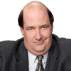
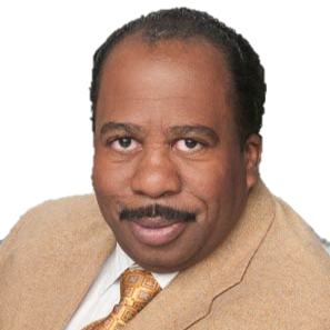
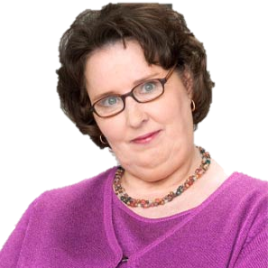
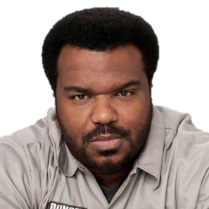
Between the main Scranton office workers (original cast, plus Andy & Erin), 94 costumes were worn over the 9 seasons. Five characters double-upped on costumes within a single episode. Oscar had an outfit change in two episodes and the most Halloween costumes throughout the series.
| Who dressed up for Halloween each season? | ||||||||||
| s1 | s2 | s3 | s4 | s5 | s6 | s7 | s8 | s9 | series | |
|---|---|---|---|---|---|---|---|---|---|---|
 |
5 | |||||||||
 |
7 | |||||||||
 |
6 | |||||||||
 |
6 | |||||||||
 |
7 | |||||||||
 |
8 | |||||||||
 |
6 | |||||||||
 |
5 | |||||||||
 |
6 | |||||||||
 |
6 | |||||||||
 |
4 | |||||||||
 |
6 | |||||||||
 |
6 | |||||||||
 |
5 | |||||||||
 |
4 | |||||||||
 |
4 | |||||||||
 |
3 | |||||||||
| A single denotes 1 costume worn in an episode. A double denotes 2 costumes. | ||||||||||
HOW TO - Represent numbers as icons & still include a summary
It was a struggle to find a concise, but visually appealing way to demonstrate who dressed up each season. I started trying to display tiny images of every costume in one table, which ended up being a headache to collect, code, and view.
Going back to basics, I decided to reproduce what I would do on an actual sheet of paper - a grid of characters by season with check marks for the data.
Two goals here:
- Be able to differentiate episodes where characters wore more than 1 costume.
- Provide summary rows with sums.
Providing a summary of the rows means that the data inside the table must be numeric, not text or html. This means I have to use the gt::text_transform() to ensure the values are changed after the summaries are calculated, rather than using dplyr::mutate() in the pre-processing. Again, I started with a function from gtExtras to make this easier.
gt_int_as_fa <- function(gt_object, column,
name = c("check", "check-double"),
palette = c("black", "red"),
threshold = 1,
...,
align = "center") {
stopifnot("Table must be of class 'gt_tbl'" = "gt_tbl" %in% class(gt_object))
text_transform(
gt_object,
locations = cells_body(columns = {{ column }}),
fn = function(x) {
int_conv <- suppressWarnings(as.integer(x))
lapply(X = int_conv, FUN = function(xy) {
# handle missing values
if(gtExtras:::is_blank(xy) || is.na(xy)){
return(gt::html(" "))
}
this_index = if(xy <= threshold){1}else{2}
this_fa <- fontawesome::fa(name[this_index], ...,
fill = palette[this_index], height = "20px", a11y = "sem") %>%
as.character() %>%
gt::html()
htmltools::div(
title = name[this_index], "aria-label" = name[this_index], role = "img",
list(this_fa)
)
})
}
) %>%
cols_align(align = align, columns = {{ column }})
}The function looks at the value of the cell. If that value is less than or equal to the threshold value of 1, it returns a single check mark fontawesome icon in black. If the value is more than the threshold, it instead returns the red double-check mark.
What did each character wear?
Another challenge is to graphically represent the diversity of costumes across the characters and seasons without overloading the table with individual photos. I assigned categories to each costume worn and then reproduce the previous table to use icons to represent those categories.
While the unique costume details are obscured, you can hover your mouse over each icon to see the details in a tooltip.
Some interesting patterns emerge from this:
- Angela consistently wears animal costumes (usually dressing as a cat).
- Jim prefers low-effort costumes, while Dwight goes for fictional characters.
- Michael generally falls into the “other” category, with his two-headed Michael costume and dick-in-a-box from SNL.
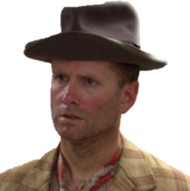
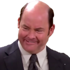
Looking at the seasons, we see that fictional characters are most popular in earlier seasons, and then there’s a shift toward real people and occupations in later seasons.
| Costumes worn in Halloween episodes, by theme | |||||||||||
| Classic: 9 total Animal: 12 Fictional character: 31 Real person: 18 Occupation: 9 Low-effort: 7 The Office universe: 4 Other: 9 Hover over an icon to see costume details |
|||||||||||
| s1 | s2 | s3 | s4 | s5 | s6 | s7 | s7 | s8 | s9 | s9 | |
|---|---|---|---|---|---|---|---|---|---|---|---|
 |
|||||||||||
 |
|||||||||||
 |
|||||||||||
 |
|||||||||||
 |
|||||||||||
 |
|||||||||||
 |
|||||||||||
 |
|||||||||||
 |
|||||||||||
 |
|||||||||||
 |
|||||||||||
 |
|||||||||||
 |
|||||||||||
 |
|||||||||||
 |
|||||||||||
 |
|||||||||||
 |
|||||||||||
 |
|||||||||||
 |
|||||||||||
 |
|||||||||||
 |
|||||||||||
| Some characters in seasons 7 and 9 wore multiple costumes. | |||||||||||
HOW TO - Represent text as icons with a tooltip
This trick is bit more involved since it involves multiple inputs:
- The table cell contents are the unique costume names. This ensures the tooltip / mouse over will have the correct name.
- An input table to relate those costume names with the costume category
- An input table to relate those categories with an icon and a color
Again, I modify the function from gtExtras to allow for these inputs and to gt::text_transform() the costume name into the html to render the icon.
category_icons <- tibble::tribble(
~costume_category, ~fa_icon, ~color,
"Classic", "ghost", "#bdda57",
"Animal", "cat", "#005452",
"Fictional character", "crown", "#d4af37",
"Real person", "user", "#4040FF",
"Occupation", "user-nurse", "#561D5E",
"Low-effort", "face-meh", "#bea493",
"The Office universe", "paperclip", "#000000",
"Other", "mask", "#444444",
)
gt_text_as_fa <- function(gt_object, column,
icon_table,
category_table,
...,
align = "center") {
stopifnot("Table must be of class 'gt_tbl'" = "gt_tbl" %in% class(gt_object))
text_transform(
gt_object,
locations = cells_body(columns = {{ column }}),
fn = function(x) {
lapply(X = x, FUN = function(xy) {
# handle missing values
if(gtExtras:::is_blank(xy) || is.na(xy)){
return(gt::html(" "))
}
this_category = category_table %>% filter(costume_detail == xy) %>% pull(costume_category)
this_icon = icon_table %>% filter(costume_category == this_category) %>% pull(fa_icon)
this_fill = icon_table %>% filter(costume_category == this_category) %>% pull(color)
this_fa <- fontawesome::fa(this_icon, ...,
fill = this_fill,
height = "20px", a11y = "sem",
title = xy) %>%
as.character() %>%
gt::html()
label <- paste(xy, this_icon)
htmltools::div(
title = xy, "aria-label" = xy, role = "img",
list(this_fa)
)
})
}
) %>%
cols_align(align = align, columns = {{ column }})
}Who dressed as each other?
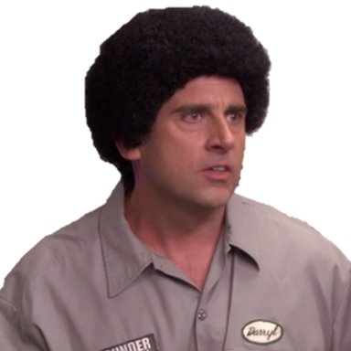
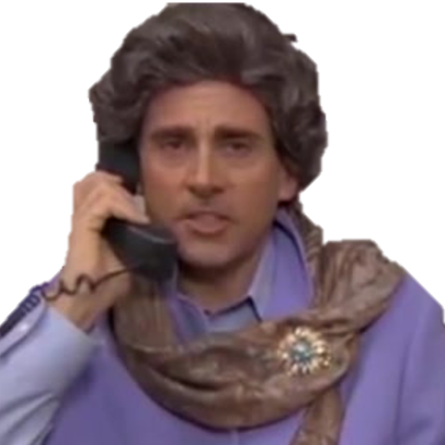
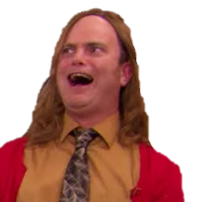
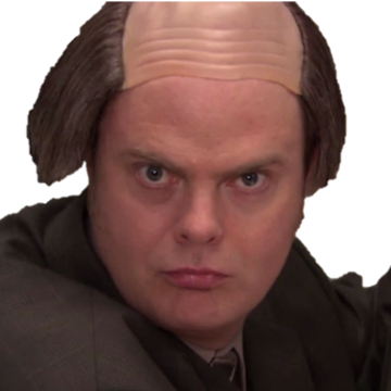
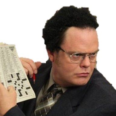
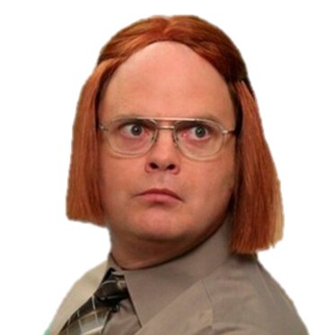
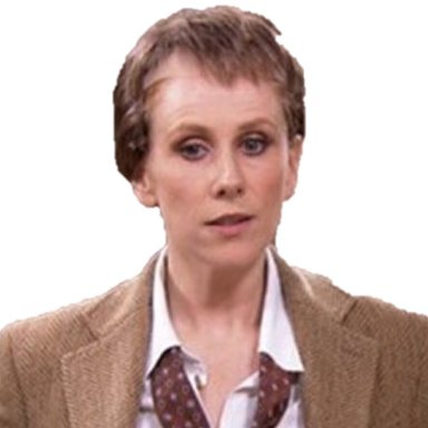
Let’s deep dive into the : The Office Universe costume category.
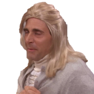
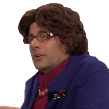
A few times in the series, characters chose to dress up as other characters from the show. It happened 3 times during Halloween, plus a few times as pranks or awkward jokes.
| Identity theft is not a joke, Jim | |||||||||||
| characters dressed up as each other | |||||||||||
| Dwight | Jim | Pam | Angela | Kevin | Stanley | Phyllis | Meredith | Darryl | Toby | Jo | |
|---|---|---|---|---|---|---|---|---|---|---|---|
 Jim |
 |
||||||||||
 Michael |
 |
 |
 |
 |
 | ||||||
 Dwight |
 |
 |
 |
 |
 |
 |
|||||
 Nellie |
 |
||||||||||
HOW TO - Custom CSS for images & combine with text
The gt helper function web_image() allows you to render a web URL of an image as an actual image in the table, with an option to set the image height but no other css.
I wanted to differentiate the row name images (the normal portraits) from the costumes using a yellow background (like sticky notes). I first customized a new web_image() function with an input more_css that takes a string of CSS, or more easily, the function css().
web_image_plus <- function(
    url,
    height = 30,
    more_css = ""
) {

  if (is.numeric(height)) {
    height <- paste0(height, "px")
  }

  paste0("<img src=\"", url, "\" style=\"height:", height, ";",
         more_css,
         "\">")
}
Tom’s gt_merge_stack() does most of the rest of the work. Instead of stacking two text cells on each other, I want to stack the output from web_image_plus() onto text (the character name). The full function is long, but you can see it here.
gt_table %>%
  gt_merge_stack_image(headshot, character_name,
                       img_height = 50,
                       img_css = css(background.color = "#ffff88",
                                     border = "solid black"))
Bonus - The Scranton Strangler
Internet fan theories are convinced that Toby is the real identity of the Scranton Strangler - the local serial killer who terrorizes Scranton by choking his victims. Toby served on the jury of the convicted Strangler but then became more obsessed with the topic toward the end of the series.
The evidence pointing to Toby is strong. In the table below, we also see that he really likes to talk about the Stangler as well - perhaps to help his ego?
| The Scranton Strangler | ||
| mentions of The Office's resident serial killer | ||
| characters | ||
|---|---|---|
 |
Dwight | |
 |
Toby | |
 |
Michael | |
 |
Andy | |
 |
Jim | |
 |
Nellie | |
| seasons | ||
| s6 | ||
| s7 | ||
| s9 | ||
HOW TO - Add blood splatter to a table
(Or how to add a watermark)
Using the gt::opt_css() function, you can add an image to the background of a gt table. I drew a blood splatter in PowerPoint, saved it as a transparent PNG, and then call that in the CSS.
When adding custom css to a gt and publishing on a webpage with multiple tables, it’s important to use the id parameter in gt::gt() and then only apply that css to that id.
Otherwise the CSS (the blood splatter in this case) will be applied to every table on the page.
data %>%
  gt::gt(id = "bloodsplatter_table") %>%
  # gt functions.... %>%
  # .... %>%
  opt_css(
    '
     #scranton_strangler table {
      background-image: url("https://raw.githubusercontent.com/ryantimpe/theoffice/master/halloween/bloodsplatter.png");
      background-repeat: no-repeat;
      background-size: 70%;
      background-position: 50% 50%;
     }
      '
  )
Code for all the tables can be found on GitHub.